SMM CME Catalog
The revised (and final) SMM CME catalog contains a description of the SMM coronagraph, an explanation of the methods used to measure CME properties, summary tables and histograms of SMM CME properties, sample images of CME morphologies, descriptions and examples of properties listed in the annual CME tables and the annual tables of all observed CMEs. For convenience we also provide a link to just the annual CME tables contained in the catalog.
Download the full SMM CME Catalog: part I, part II.
You may also download just the CME event tables and trajectory files by year (in PDF format):
1980
1984
1985
1986
1987
1988
1989
Using the CME Catalog and Accompanying CME Trajectory Files
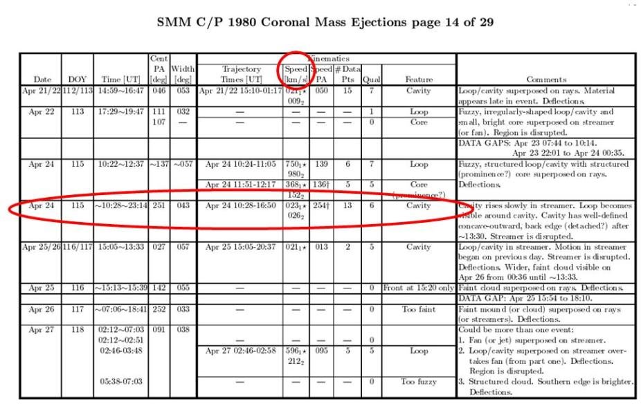
Figure 1. An example of the SMM CME catalogue from 1980. Basic CME information (except start times) are provided.
SMM CME basic properties such as speeds, locations and widths are provided in the SMM CME catalogue (except start times). An example from 1980 is shown in Figure 1. For many CMEs it was possible to track at least one feature and produce a time-height trajectory to provide a constant speed (first order polynomial), and for events with more than 2 data points a constant acceleration (second order polynomial). In most cases both the constant speed (subscript 1) and final speed (subscript 2) from the constant acceleration fit are reported. A preferred speed is indicated by an ‘*’ based on a chi-squared analysis of the fits and a visual inspection of the trajectories. When a CME has a constant velocity preferred fit, the acceleration measurement is considered to be insignificant and therefore unmeasurable.
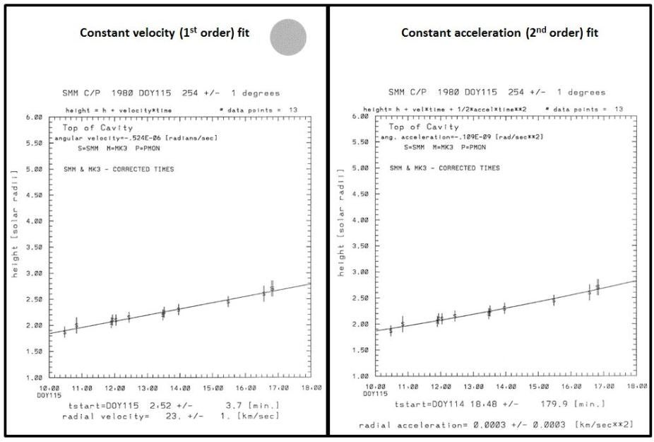
Figure 2. Plots of CME trajectories from April 24 (DOY 115) 1980. At left is a constant velocity (1st order fit) and at right is a constant acceleration (2nd order fit) to the CME cavity feature. The dot at the top of the constant velocity plot on the left indicates this is the preferred fit.
We have recently digitized all the SMM CME trajectories and have made them available online. The trajectories provide additional information, such as projected CME start times, that are not available in the catalogue. Figure 2 displays the trajectory of the April 24, 1980 10:28 CME that is highlighted by the red oval in Figure 1. The preferred speed is indicated on the trajectory by a large dot at the top of the plot. Information files accompany each trajectory and contain the time-height measurements and the trajectory fitting information including: the projected CME start time at 1 solar radii, or at the height , the constant speed (1st order fits), the acceleration (2nd order fits), the speed at each data point, the coefficients of the fit and the goodness of the fit.
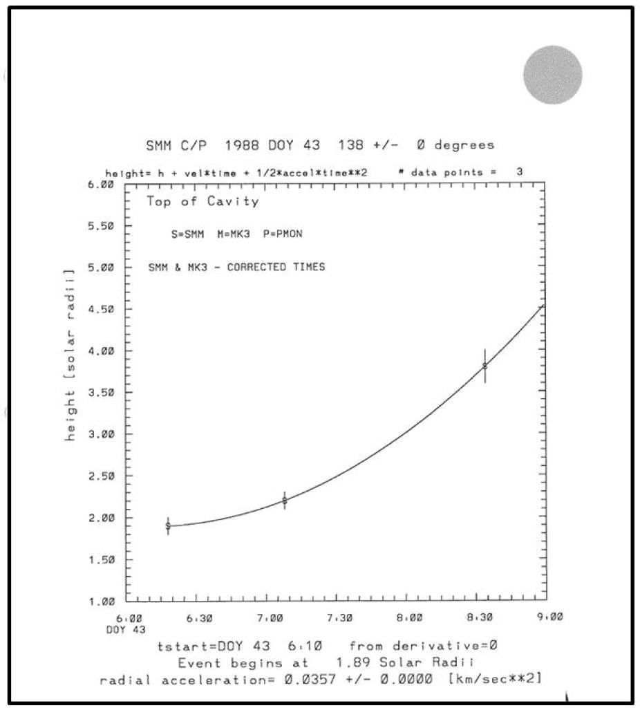
Figure 3. A CME trajectory from 1988 DOY 43 (Feb 12). The parabolic fit to the data does not intersect the height of 1 solar radii. The height of the parabola vertex, in this case 1.89 solar radii, is used to determine the CME start time. Both the start time and the height are reported in the trajectory plot.
The estimated start time of the CME at 1 solar radii is provided at the bottom of the plots. Some second order fits (e.g. a parabola) lie entirely above the height value of 1 solar radii. In those cases the lowest height of the parabola is reported (height > 1 solar radii) and the CME can be considered to have been accelerated from a height above 1 solar radii in the corona. An example of such a trajectory is shown in Figure 3. For additional information, please see the SMM CME catalogue.
Reference: A Revised and Expanded Catalogue of Mass Ejections Observed by the Solar Maximum Mission Coronagraph (J.T. Burkepile and O.C. St.Cyr).
The catalogue was published by the National Center for Atmospheric Research (NCAR); Technical Note Number NCAR / TN-369+STR (1993).
SMM Data Use Policy
The use of SMM C/P images for public education efforts and non-commercial purposes is strongly encouraged and requires no expressed authorization. However, it is requested that any such use properly attributes the source of the images as: "Courtesy of HAO/SMM C/P project team & NASA. HAO is a division of the National Center for Atmospheric Research, which is supported by the National Science Foundation."
Acknowledgements
The Solar Maximum Mission Coronagraph/Polarimenter was designed & operated by the High Altitude Observatory, a division of the National Center for Atmospheric Research, and funded by the National Science Foundation. The SMM Coronagraph/Polarimeter instrument was built by Ball Aerospace Systems Division. The SMM Spacecraft was built by Goddard Space Flight Center, and the SMM project was funded & managed by the National Aeronautics & Space Administration.