Spectral Line Inversions
Spectral lines carry a wealth of information on the physical properties of the medium in which they were formed. This information is encoded in the subtle details of their shape and their state of polarization. Spectral line inversion codes are tools designed to decipher this information, allowing one to extract the physical properties of the medium (atmosphere) in which the lines are formed.
Inversion codes typically have two distinct components: one that carries out the forward modeling of the spectral line, and another one that deals with the inversion problem itself. Several different approaches exist to tackle each one of these.
The Forward Problem
The forward problem consists of finding the solution to the Radiative Transfer Equation (RTE) given the physical conditions of the atmosphere and a set of assumptions that determine the behavior of the light as it travels through the medium. The solution to the RTE is the spectrum of the intensity and polarization of the light. In terms of physical understanding, it is in these assumptions where the difference among the available codes stems. Broadly speaking, one can encounter three different approaches, listed here in order of increasing complexity:
- The Milne-Eddington (ME) approximation makes the assumption that the properties of the atmosphere are constant with height, except for the source function, which is allowed to vary linearly with optical depth. Most of the parameters of the model atmosphere serve the purpose of parametrizing the shape of the spectral line, and don’t translate directly into thermodynamical physical quantities such as density or temperature.
- The LTE (Local Thermodynamical Equilibrium) approximation assumes that the populations of the energy levels of the atoms depend only on the local values of temperature and density. Under this assumption, the RTE can still be solved analytically. Actual thermodynamical magnitudes (rather than parameters that describe the shape of the spectral line) go into the mathematical formulation and become an output of the spectral line inversion.
- Non-LTE solutions to the RTE can be more or less comprehensive in the details of the physical modeling of particle-radiation interaction. They all have in common, however, that they take into account the non-local interaction between matter and light. The populations of the energy levels of the atoms are obtained by solving the Statistical Equilibrium Equations (SEE) which, in turn, depend on the solution of the RTE, and vice-versa. This is a complex non-linear problem that does not have an analytical solution. Different numerical techniques have been developed to tackle this problem in an iterative manner in order to find a self-consistent solution in the least amount of time.
Generally speaking, the ME and LTE assumptions are valid in the Photosphere, whilst the general non-LTE formulation is necessary to interpret Chromospheric radiation. However, the ME approach is not able to reproduce asymmetries in the spectral line morphology. Figure 1 (courtesy of R. Casini) shows a schematic of the general inversion problem. The green-shaded area encompasses the full forward calculation, which requires solving the radiative transfer and the statistical equilibrium equations in a self-consistent manner. As the arrows indicate, the solution to each one of these feeds back into the other.
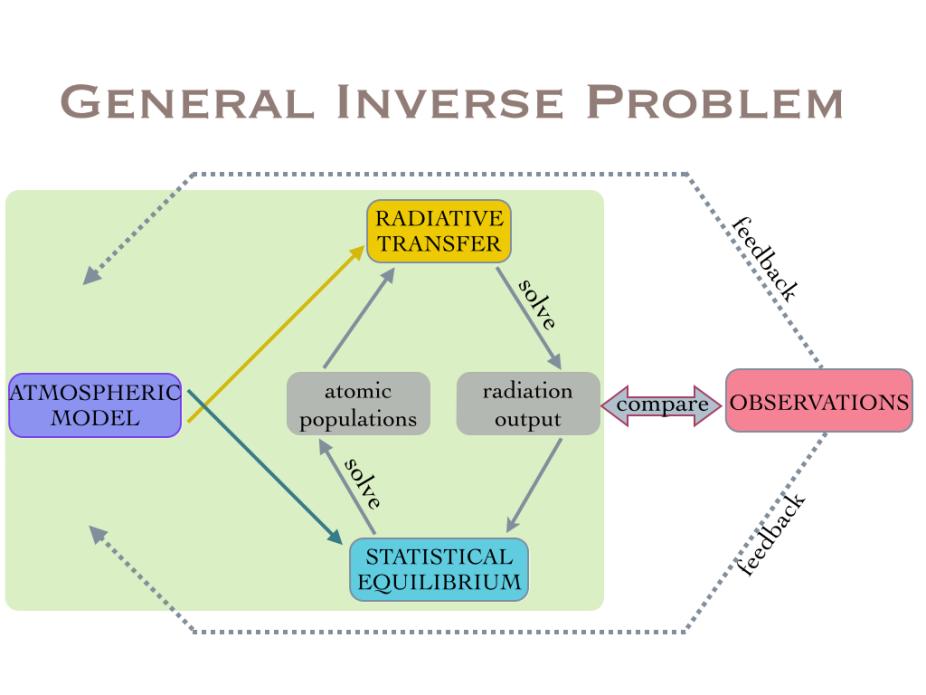
General inverse problem flowchart
The Inverse Problem
The inversion problem has the opposite goal to the forward modeling: given a spectral line, its objective is to calculate the physical properties of the atmosphere in which the light was generated. The inversion strategy will be coupled to one of the forward modeling approaches and its job is to find the combination of physical parameters (in the context of the chosen model atmosphere) that best reproduce the observed spectral line profiles. Several approaches can be used to tackle the inversion problem. They can often be categorized in one of the following:
- Least Squares Minimization algorithms: the objective of these methods is to minimize a merit function that quantifies the quality of the fit between the observed and the synthetic spectral lines. Inversion codes based on these minimization schemes need an initial guess for the model atmosphere. Then they carry out the forward modeling to create a set of synthetic Stokes profiles that are compared to the observed ones. If the fit isn't deemed to be good enough, the algorithm will tweak the parameters of the model atmosphere and compute the synthetic spectral line once again. This process will be repeated in an iterative manner until the synthetic and the observed spectra match in a least squares sense. Often, Levenberg-Marquardt least squares minimization techniques are used for this task. The inherent iterative nature of these algorithms makes them slow (depending on how computationally intensive the forward modeling is), and the risk of falling into a local minimum of the merit function is dependent on the initialization. However, once they are on the right converging path, they are very effective at finding an accurate solution.
- Pattern recognition techniques: these techniques rely on the creation of a database of spectral profiles that covers the parameter space of the atmospheric model. The observed spectrum is then compared against the profiles in the database and a metric of similarity is used to find the best fit amongst the synthetic profiles. Thee strength of these methods lies in that they are better at finding a global solution. They are also significantly faster than the Least Squares fitting procedures. The main disadvantage of these methods is that the solution found by the inversion is as precise as the sampling of the model parameters used to create the database. The finer the sampling, the more precise the solution, but also the larger and more unmanageable the database will be.
Inversion codes
CSAC has compiled a number of community spectral line inversion codes that use different forward modeling assumptions and different inversion strategies. You can find them here.