Modeling high-speed flows in the Earth’s Magnetotail
The magnetosphere is created by the interaction between the solar wind and the Earth’s magnetic field. On the dayside of the Earth pressure from the solar wind compresses the Earth’s dipole magnetic field and on the night side this interaction stretches it out forming a region of space commonly referred to as the magnetotail. Depending on the direction of the magnetic field in the solar wind, mass, momentum, and energy can be transferred into the magnetotail making it a highly dynamic region full of high-speed plasma flows. HAO scientist Michael Wiltberger, working with colleagues at Dartmouth College and John’s Hopkin’s University, used the Lyon-Fedder-Mobarry global magnetosphere model in its highest resolution mode to simulate these dynamic flows.
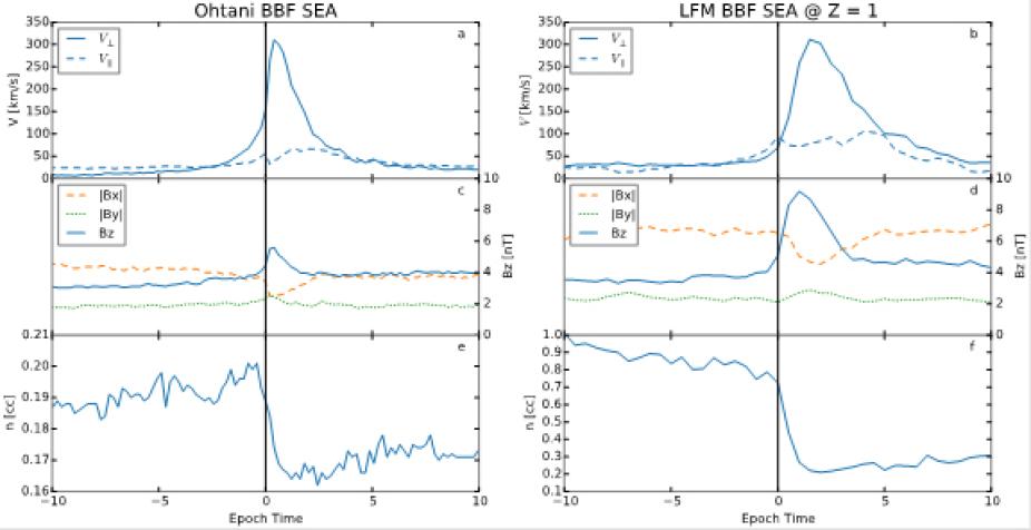
Figure 1: Wiltberger, M., V. Merkin, J. G. Lyon, and S. Ohtani (2015), High-resolution global magnetohydrodynamic simulation of bursty bulk flows, J. Geophys. Res., 120(6), 4555–4566, doi:10.1002/2015JA021080.
Figure 1 shows a scientific visualization of the magnetotail as the interplanetary magnetic field (IMF) goes from northward to southward. Southward IMF allows for the most energy transfer from the solar wind into the magnetosphere. The visualization shows the magnetotail with a colored plane cut through the center of the Earth. On this plane the difference between dipole magnetic field and the current value is illustrated with the green/purple color scheme. You can see the compression of the Earth’s dipole field on the dayside at the beginning of the movie. As the movie progresses, the magnetotail becomes dominated by numerous high-speed flows that propagate from the further down the tail towards the Earth. The colored arrows in the visualization illustrate the strength and direction of these flows. A larger redder arrow represents stronger flows. The green concave feature at the leading of these flows represents a compression of the magnetic field. This compression returns the field to a more dipolar magnetic field configuration and is the origin of the name dipolarization fronts that scientists use for these features.
These dipolarization fronts are often observed in the magnetotail by various NASA spacecraft. A challenge in comparing these observations with the simulation results is that because the flow is nearly turbulent it is difficult if not impossible to have the spacecraft exactly the same spot in the real magnetotail and the simulation. The investigators overcome this challenge by making a statistical comparison between the observed flows and the simulation results. Figure 2 illustrates the results of using the same selection criteria to observe high-speed flows in the simulation and real magnetotail. On the left hand side of Figure are results for the flow speed, magnetic field, and density observed by the Geotail mission while it was in the magnetotail. On the right hand side are results from the high-resolution LFM simulation. The flows show a slightly broader profile than the observations with similar peak value. The magnetic field shows the compression of the BZ field in both the simulation and observations. There is a density drop in both sets of data, but the magnitude is much larger in the simulated results. This is likely due to the preconditioning of the magnetosphere in the simulation. In general, these results are in good agreement and provide verification that the high-resolution simulations are doing a good job of capturing the dynamics of the magnetotail.