Astrophysical Journal: Inferring the three-dimensional (3D) solar atmospheric structures from observations is a critical task for advancing our understanding of the magnetic fields and electric currents that drive solar activity. In this work, we introduce a novel, Physics-Informed Machine Learning method to reconstruct the 3D structure of the lower solar atmosphere based on the output of optical depth sampled spectropolarimetric inversions, wherein both the fully disambiguated vector magnetic fields and the geometric height associated with each optical depth are returned simultaneously. Traditional techniques typically resolve the 180-degree azimuthal ambiguity assuming a single layer, either ignoring the intrinsic non-planar physical geometry of constant optical-depth surfaces (e.g., the Wilson depression in sunspots), or correcting the effect as a post-processing step. In contrast, our approach simultaneously maps the optical depths to physical heights, and enforces the divergence-free condition for magnetic fields fully in 3D. Tests on magnetohydrodynamic simulations of quiet Sun, plage, and a sunspot demonstrate that our method reliably recovers the horizontal magnetic field orientation in locations with appreciable magnetic field strength. By coupling the resolutions of the azimuthal ambiguity and the geometric heights problems, we achieve a self-consistent reconstruction of the 3D vector magnetic fields and, by extension, the electric current density and Lorentz force. This physics-constrained, label-free training paradigm is a generalizable, physics-anchored framework that extends across solar magnetic environments while improving the understanding of various solar puzzles.
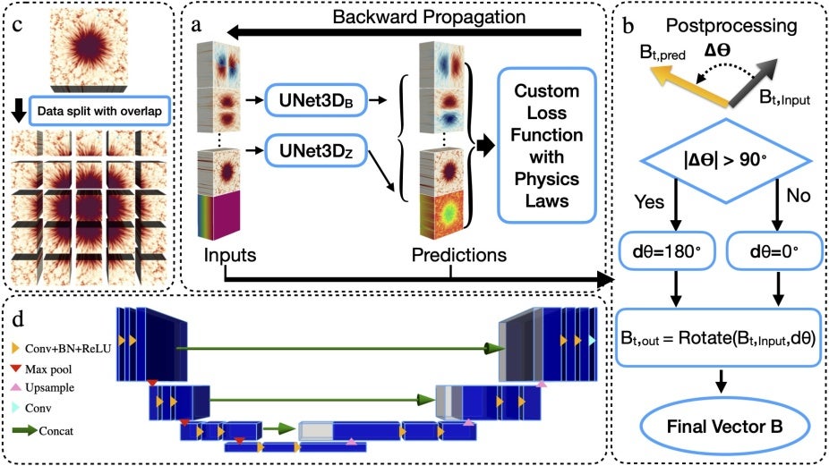
Panel (a) shows the flowchart for training the model. The inputs are the 3D magnetic vector fields with azimuthal ambiguity, and an initial guess of the geometric heights associated with each optical-depth layer. The UNet3DB network predicts 3D vector magnetic field, and the UNet3DZ network provides the geometric heights. They are combined to compute a custom loss function that also considers physical constraints (divergence free magnetic field). Panel (b) shows the post-processing step that assembles the outputs from the neural networks (prediction) and the original input magnetic fields into the final output. Panel (c) shows an example of the 3D data, split with overlaps between nearby subfields. These individual subfields are used as the input for training. Panel (d) presents the UNet3D structure, reproduced from Figure 2 in Cicek et al. (2016).