Solar Physics Historical Timeline (1800-1999)
Timeline
In this page
1800: The Sun's invisible radiation
Herschel's experimental setup for the detection of invisible solar radiation. Sunlight passes through a prism, forming the usual rainbow spectrum. A row of thermometers is positioned on a table beyond the red end of the spectrum. Thermometer 1, aligned with the spectrum, registers a rise in temperature, while the control thermometers 2 and 3 do not.
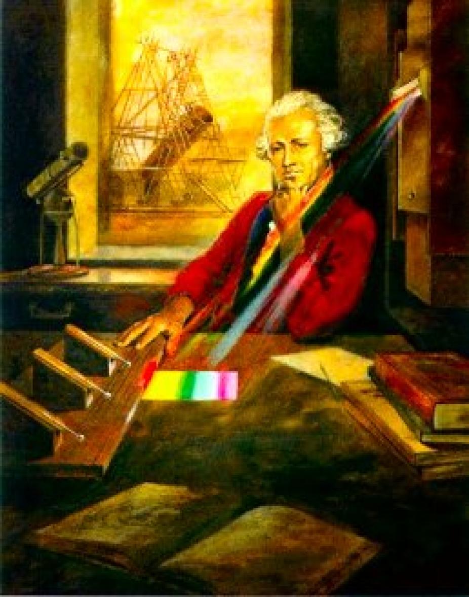
In the 1660's Isaac Newton had shown that sunlight can be separated into separate chromatic components via refraction through a glass prism. In 1800, William Herschel extended Newton's experiment by demonstrating that invisible "rays" existed beyond the red end of the solar spectrum. He did so by detecting the temperature rise in thermometers placed beyond the red end of the visible solar spectrum.
Herschel boldly conjectured that these invisible caloric rays, later named infrared radiation, were fundamentally no different from visible light, and could not be seen simply because the eye is not sensitive to them. Herschel also sought caloric rays beyond the violet end of the spectrum, but to no avail. However, the following year, Johann Wilhelm Ritter (1776–1810) used an experimental setup similar to Herschel's, but placed beyond the violet end of the spectrum a piece of paper soaked in silver chloride; the subsequent blackening of the paper beyond the visible violet demonstrated the existence of ultraviolet radiation. The following year, and using similar photochemical means, William Hyde Wollaston (1766-1828) independently rediscovered ultraviolet radiation.
References and further readings
- Herschel, W. 1800, Experiments on the Refrangibility of the Invisible Rays of the Sun, Philosophical Transactions of the Royal Society of London 90, 284-292
- Meadows, A.J. 1970, Early Solar Physics, Pergamon Press.
1802: Black lines in sunlight
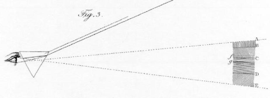
Wollaston's experimental setup for the prismatic observation of the solar spectrum. Wollaston believed that the lines labeled here B, C and E marked natural color boundaries, although he also noticed other dark lines (f,g) that did not appear to delineate colors.
Reproduced from Philosophical Transactions of the Royal Society of London, vol. 92 (1802), p. 380 (Plate XIV)
While investigating the refractive properties of various transparent substances, the English chemist and physicist William Hyde Wollaston noticed dark lines in the spectrum of the Sun as viewed through a glass prism following the method of Isaac Newton. Beyond suggesting that these dark lines marked the boundaries of "natural colors," Wollaston did not pursue the matter much further. Yet this marked the first step towards solar spectroscopy, which was to revolutionize Solar Physics in the second half of the century.
References and further readings
- Wollaston, W. H. 1802, A Method of Examining Refractive and Dispersive Powers by Prismatic Reflection, Philosophical Transactions of the Royal Society of London 92, 365-380
- Meadows, A.J. 1970, Early Solar Physics, Pergamon Press.
1817: Solar spectroscopy is born

Reproduction of Fraunhofer's original 1817 drawing of the solar spectrum. The more prominent dark lines are labeled alphabetically; some of this nomenclature has survived to this day.
Denkschriften der K. Acad. der Wissenschaften zu München 1814-15, pp. 193-226
In what was to later lead to some of the more important advances in solar physics, Joseph von Fraunhofer (1787–1826) independently rediscovered the "dark lines" in the solar spectrum noticed 15 years earlier by William Hyde Wollaston. Fraunhofer pursued the matter mainly because he saw the possibility of using the lines as wavelength standards to be used to determine the index of refraction of optical glasses. Other physicists, however, were quick to realize that the Fraunhofer lines could be used to infer properties of the solar atmosphere, as similar lines were also observed in the laboratory in the spectrum of white light passing through heated gases.
In the hands of David Brewster (1781-1868), Gustav Kirchhoff (1824-1887), Robert Wilhelm Bunsen (1811–1899), and Anders Jonas Ångström (1814-1874) to name a few, spectroscopy turned into a true science which revolutionized not only solar physics, but also astronomy at large. Even today, most information gathered on the Sun and stars is obtained through spectroscopic means.
References and further readings
- Meadows, A.J. 1970, Early Solar Physics, Pergamon Press.
1838: The solar constant
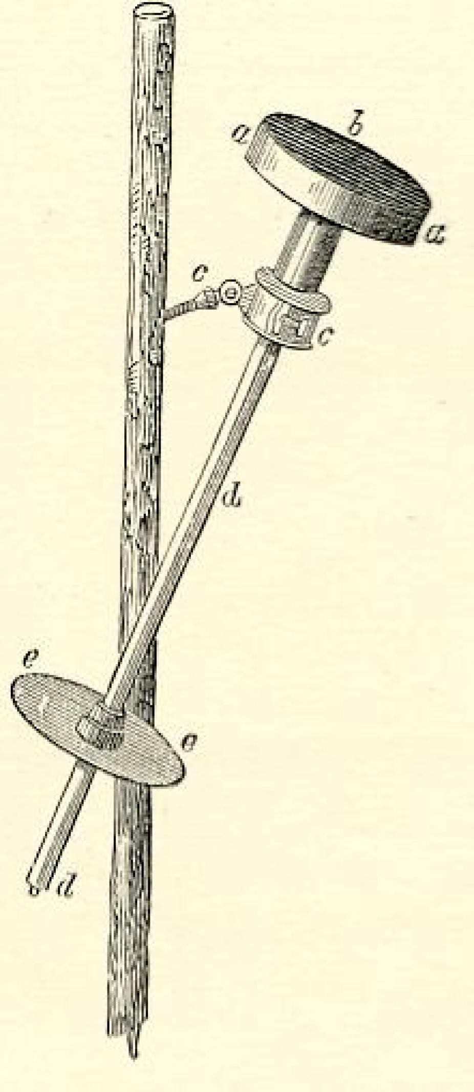
Pouillet's pyrheliometer.
The solar constant is a measure of the sun's luminosity, and is defined as the amount of solar energy per second falling on one square meter of the Earth's outer atmosphere, when the Earth is at a distance of exactly one astronomical unit (149,598,500 km) from the Sun. Although various scientists had attempted to calculate the Sun's energy output, the first attempts at a direct measurement were carried out independently, and more or less simultaneously, by the French physicist Claude Pouillet (1790–1868) and British astronomer John Herschel (1792–1871). Although they each designed different apparatus, the underlying principles were the same: a known mass of water is exposed to sunlight for a fixed period of time, and the accompanying rise in temperature recorded with a thermometer. The energy input rate from sunlight is then readily calculated, knowing the heat capacity of water. Their inferred value for the solar constant was about half the accepted modern value of 1367 ± 4 Watt per square meter, because they failed to account for of absorption by the Earth's atmosphere.
Pouillet's instrument (shown here) depicts water contained in the cylindrical container a, with the sun-facing side b painted black. The thermometer d is shielded from the Sun by the container, and the circular plate e is used to align the instrument by ensuring that the container's shadow is entirely projected upon it. Reproduced from A.C. Young's The Sun (revised edition, 1897).
References and further readings
- Young, C.A. 1897, The Sun (revised ed.), Appleton and Co., chap. 8
- Hufbauer, K. 1991, Exploring the Sun, The Johns Hopkins University Press.
1843: The sunspot cycle
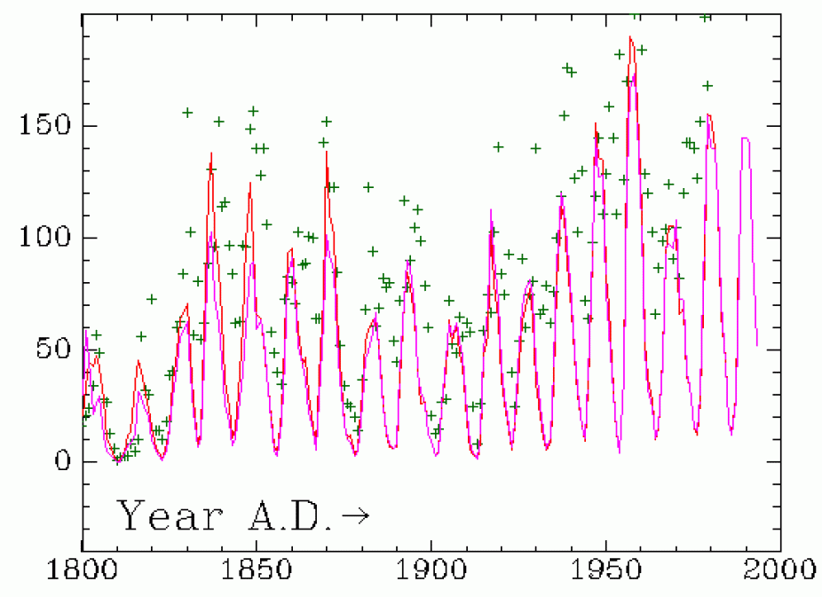
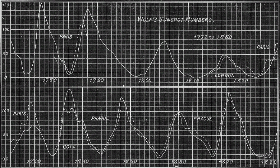
Variation in observed sunspot numbers during the time period 1800-2000. The red curve is the Wolf sunspot number, and the purple line a count of sunspot groups based on a reconstruction by D.V. Hoyt. The green crosses are auroral counts, based on a reconstruction by K. Krivsky and J.P. Legrand.
Early sunspot observers noted the curious fact that sunspots rarely appear outside of a latitudinal band of about ± 30° centered about the solar equator, but otherwise failed to discover any clear pattern in the appearance or disappearance of sunspots. In 1826, the German amateur astronomer Samuel Heinrich Schwabe (1789–1875), set himself the task of discovering intra-mercurial planets, whose existence had been conjectured for centuries. Like many before him, Schwabe realized that his best chances of detecting such planets lay with the observation of the apparent shadows that they would cast while crossing the visible solar disk during their transit. The primary difficulty with this research program was the ever-present danger of confusing such planets with small sunspots. Accordingly, Schwabe began recording very meticulously the position of any sunspot visible on the solar disk on any day that weather would permit solar observation. In 1843, after 17 years of observations, Schwabe had not found a single intra-mercurial planet, but had discovered something else of great importance: the cyclic increase and decrease with time of the average number of sunspots visible on the Sun, with a period that Schwabe originally estimated to be 10 years, only one year shorter than the actual value.
References and further readings
- Stix, M. 1989, The Sun, Springer.
1845: The first solar photograph
The first photographic technique was developed in the 1830's by J. N. Niépce (1765–1833) and Louis Daguerre (1789–1851), which relied on the exposure of a thin iodine layer deposited on a silver substrate, subsequently fixed in a mercury bath. The images so produced became known as "daguerrotypes". This imaging technique was very soon applied to astronomy, through the enthusiastic support of the French astronomer and politician Francois Arago (1786–1853) and the British astronomer John Herschel, who first coined the term "photography", as well as "positive" and "negative" images.
Reproduction of the first daguerrotype of the Sun. The original image was a little over 12 centimeters in diameter.
Reproduced from G. De Vaucouleurs, Astronomical Photography, MacMillan, 1961 [plate 1]
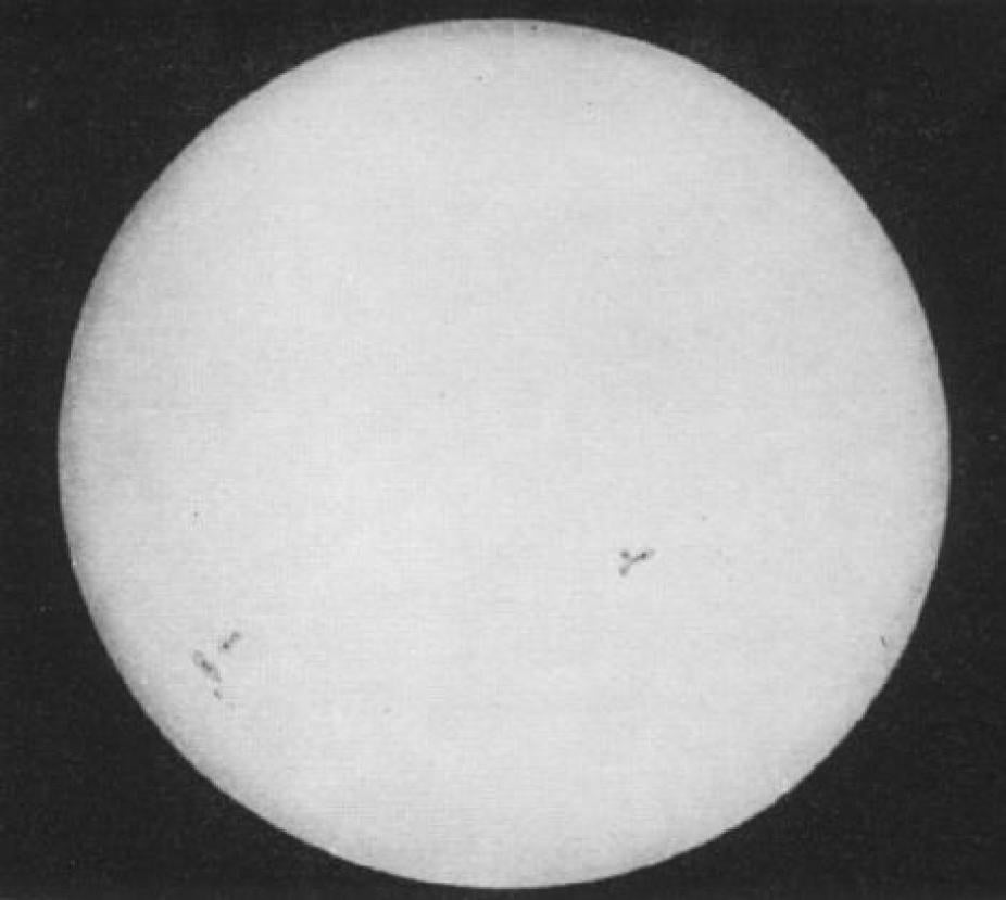
The first successful daguerrotype of the Sun, shown here, was made on 2 April 1845 by the French physicists Louis Fizeau (1819–1896) and Léon Foucault (1819–1868), both being perhaps better known for their various pioneering measurements of the speed of light. The exposure was 1/60 of a second. This image shows the umbra/penumbra structure of sunspots, as well as limb darkening.
Daguerre's photographic process was soon supplanted by a new technique (developed starting in 1851) based on a colloidal suspension on a glass substrate, in essence the direct ancestor of modern photographic film. In 1858, daily photographic recording of the solar disk using a solar telescope especially designed for photography began at Kew, England, under the leadership of Warren De la Rue (1815–1889). Photographic techniques were soon thereafter applied to the study of prominences, solar granulation, and solar spectroscopy, with some of the more spectacular results of the period obtained by Jules Janssen (1824–1907) at Meudon, near Paris. The first photograph of a solar prominence was captured by Charles A. Young (1834–1908) in 1870.
The first useful Daguerrotype of a solar eclipse was secured on 28 July 1851 by the photographer/astronomer Berkowski at the Königsberg observatory (then in Prussia, now Kaliningrad in Russia). De la Rue's group also obtained many fine photographs of the 18 July 1860 total eclipse in Spain. Eclipse photographic techniques were further improved by the introduction of radial gradient filters, designed to differentially attenuate the innermost, brightest portion of the corona. The resulting photographs allow to discern details of coronal structure out to many solar radii; see for example slide 9 and slide 10 of the HAO slide set.
References and further readings
- De Vaucouleurs, G. 1961, Astronomical Photography, New York: MacMillan.
- Lankford, J. 1984, The impact of photography on astronomy, in The General History of Astronomy, vol. 4A, ed. O. Gingerich, Cambridge University Press, pps. 16–39.
1848: The sunspot number
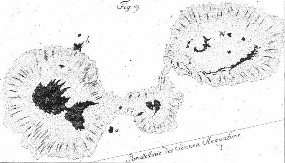
Sunspot drawings by Johann Hieronymus Schroeter (1745–1816), an active solar observer between 1785 and 1795. Schroeter's sunspot drawings were a primary source for Wolf's reconstruction of activity cycle number 4 (1785–1798).
As Schwabe's discovery of the sunspot cycle gained recognition, the question immediately arose as to whether the cycle could be traced farther into the past on the basis of extant sunspot observations. In this endeavor the most active researcher was without doubt the Swiss astronomer Rudolf Wolf (1816–1893). Faced with the daunting task of comparing sunspot observations carried out by many different astronomers using various instruments and observing techniques, Wolf defined the relative sunspot number (r) as follows:
r=k(f+10g)
where g is the number of sunspots groups visible on the solar disk, f is the number of individual sunspots (including those distinguishable within groups), and k is a correction factor that varies from one observer to the next (with k=1 for Wolf's own observations, by definition). This definition is still in use today, but r is now usually called the Wolf (or Zürich) sunspot number. Wolf succeeded in reliably reconstructing the variations in sunspot number as far back as the the 1755–1766 cycle, which has has since been known conventionally as "Cycle 1," with all subsequent cycles numbered consecutively thereafter.
References and further readings
- Hoyt, D.V. & Schatten, K.H. 1997, The Role of the Sun in Climate Change, Oxford University Press.
- Hoyt, D.V. & Schatten, K.H. 1998, Group sunspot numbers: a new solar activity indicator, Solar Physics, 181, 491–512.
1852: The sunspot cycle is linked to geomagnetic activity
The correlation between sunspot number and geomagnetic activity index.
Diagram reproduced from A.C. Young's 'The Sun' (revised edition, 1897)
In 1852, within a year of the publication of Schwabe's results in Kosmos, Edward Sabine (1788–1883) announced that the sunspot cycle period was "absolutely identical" to that of geomagnetic activity, for which reliable data had been accumulated since the mid-1830s. In fact, three other researchers arrived at the same conclusion independently, and more or less simultaneously: Rudolf Wolf and Jean-Alfred Gautier (1793–1881), both in in Switzerland, and Johann von Lamont (1805–1879) in Germany. This marked the beginning of solar-terrestrial interaction studies.
References and further readings
- Hoyt, D.V. & Schatten, K.H. 1997, The Role of the Sun in Climate Change, Oxford University Press.
- Kivelson, M.G., and Russell, C.T. (eds.) 1995, Introduction to Space Physics, Cambridge University Press, chap. 1.
1858–1859: The Sun's differential rotation
Early nineteenth century solar astronomers were increasingly intrigued at the fact that determinations of the solar rotation period obtained by tracking sunspots, carried out over the preceding two centuries, varied between anywhere from 25 to 28 days. This difference, while small, was significantly larger than the accuracy with which good observers could track sunspot motion.
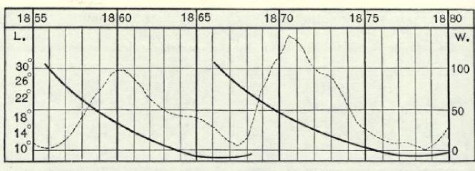
Spörer's Law of sunspot migration. The thick lines shows the latitude at which most sunspots are found (vertical axis, equator is at zero), as a function of time (horizontal axis). The dashed line is the Wolf sunspot number, showing the rise and fall of the solar cycle.
The resolution of this puzzle came in 1858, when Richard C. Carrington (1826–1875) in England and, shortly thereafter, Gustav Spörer (1822–1895) in Germany independently made two key discoveries. First, the latitude at which sunspots are most often seen decreases systematically from about 40° to 5° latitude as the sunspot cycle proceeds from one minimum to the next. Second, sunspots located at higher latitudes are carried around the sun more slowly than spots at lower latitudes. From this, Carrington concluded that the Sun rotates "differentially", yet another argument in favor of the fluid or gaseous nature of the Sun's outer layers. The aforementioned historical discrepancies in the solar rotation period are then explained by the fact that different astronomers simply observed the Sun at different epochs of the cycle.
The rapid development of spectroscopic techniques in the second half of the nineteenth century offered another means of measuring the surface differential rotation, one that is not restricted to latitudes where sunspots are present: measurement of the wavelength shift of spectral lines between the approaching and receding solar limbs, as a consequence of the Doppler effect. This was first carried out by Hermann Vogel (1841–1907) in 1871, and a few years after by Charles Young. These results were accurate enough to demonstrate that sunspots rotate at very nearly the same rate as the sun's photosphere. By the late 1880's Nils Dúner (1839–1914) had secured accurate spectroscopic rotational period calculations at latitudes about twice higher than the sunspot belts, demonstrating that the Sun's polar regions rotate about 30% slower than its equator.
Interestingly, Christoph Scheiner had already noted in his 1630 Rosa Ursina that the rotation period inferred from tracking sunspots at different heliocentric latitudes showed a systematic increase with latitude. However, in Scheiner's Aristotelian framework, the Sun could only be a solid, rigidly rotating sphere, and therefore he interpreted his data as a proof that sunspots were not markings on the solar surface, but instead cloud-like structures floating above it, since a fluid Sun was "physically absurd". For this reason, most historians of science continue to attribute the discovery of solar differential rotation to Carrington and Spörer.
References and further readings
- Mitchell, W.M. 1916, The History of the Discovery of Solar Spots, Popular Astronomy, 24, 22–ff.
- Eddy, J.A., Gilman, P.A., and Trotter, D.E. 1977, Science, 198, 824–829.
1859: First observation of a solar flare
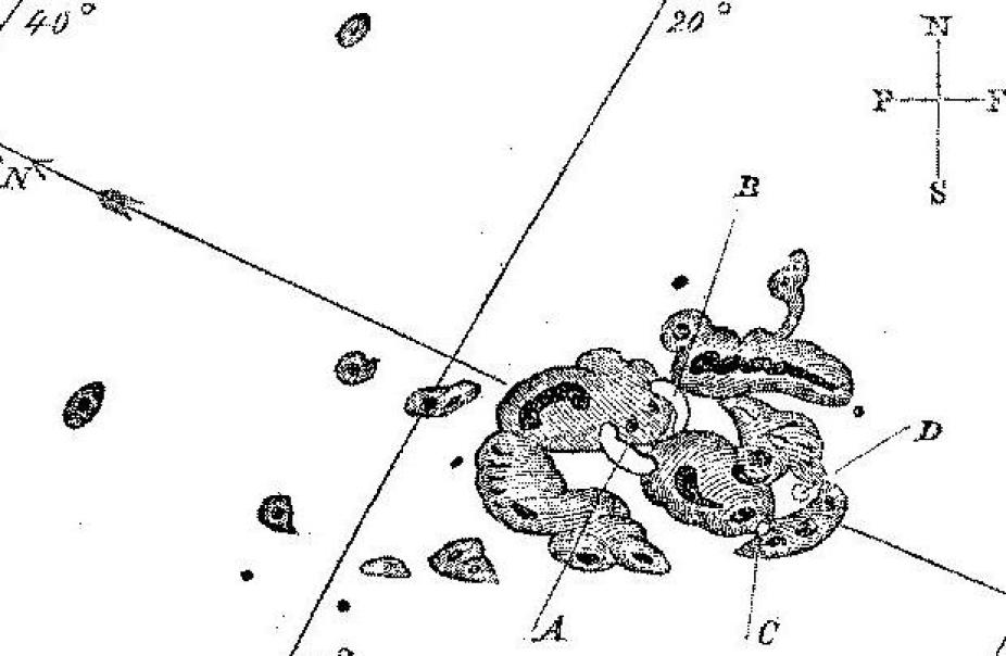
Reproduction of a drawing by R.C. Carrington, showing the location of the flare he observed while making a drawing of an active region.
Reproduced from his 1860 paper in Monthly Notices of the Royal Astronomical Society (vol. 20, p. 13)
On 1 September 1859, the amateur astronomer Richard C. Carrington was engaged in his daily monitoring of sunspots when he noticed two rapidly brightening patches of light near the middle of a sunspot group he was studying (indicated by A and B on the drawing shown here). In the following minutes the patches dimmed again while moving with respect to the active region, finally disappearing at positions C and D. This unusual event was also independently observed by R. Hodgson (1804–1872), another British astronomer.
This serendipitous observation represents the first clear description of a solar flare, corresponding to a sudden and intense heating of solar atmospheric plasma caused by reconnection of magnetic fields. What Carrington observed would today be called a two-ribbon flare. Only the largest flares are bright enough to be seen in visible light. They are readily seen in X-rays, however (see slide 15 of the HAO slide set). An earlier, plausible observational report of a white light flare has been found in the (unpublished) notebooks of the English scientist and amateur astronomer Stephen Gray (1666–1736), who on 27 December 1705 observed what he described as a "flash of lightning" near a sunspot.
Both Carrington and Hodgson noted that magnetic monitoring instruments registered strong disturbances at about the same time, but it is not possible to tell for sure whether these were due to the flare they actually saw. It is more likely that they were caused by other generalized solar disturbances of which the flare was but one manifestation.
References and further readings
- Carrington, R.C. 1860, Monthly Notices of the Royal Astronomical Society, 20, p. 13.
- Lang, K.R. 2000, The Sun from Space, Springer, chap. 6
1859: The chemical composition of the Sun
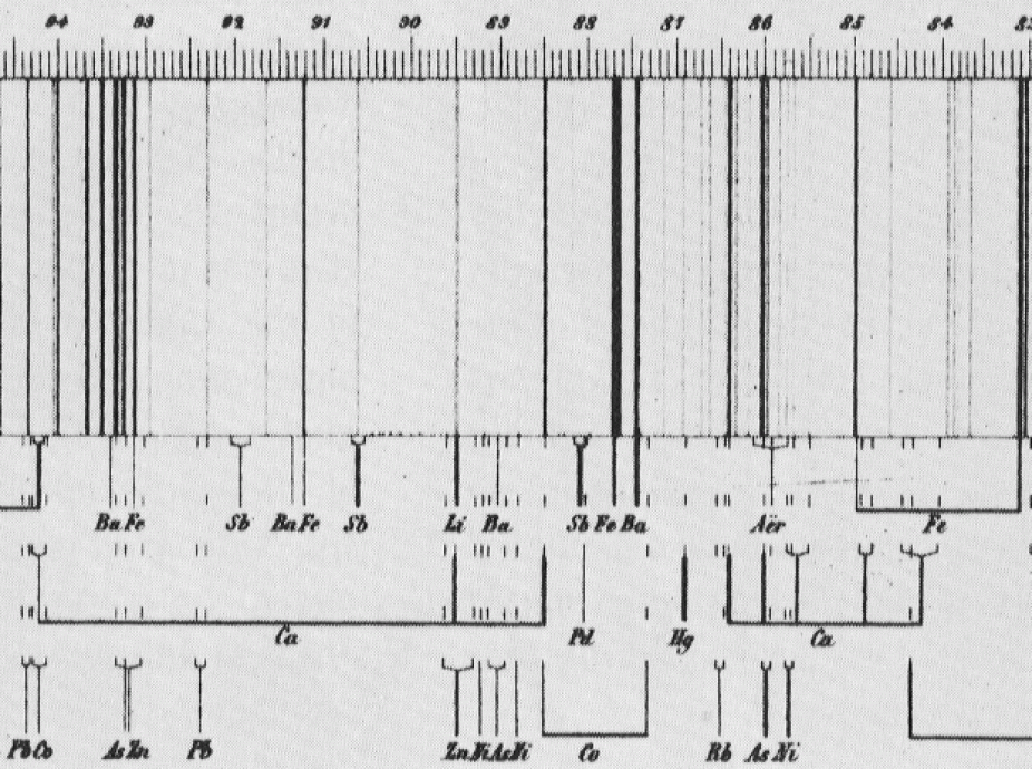
Reproduction of part of the map of the solar spectrum published in 1863 by Kirchhoff, showing the identification of a large number of spectral lines with various chemical elements. Note numerous clear matches for Iron (Fe).
In the late 1850s the chemist Robert Wilhelm Bunsen (1811–1899) and theoretical physicist Gustav Kirchhoff, both at Heidelberg, took on the issue of spectral line identification where Joseph von Fraunhofer had left it some 40 years earlier. By simultaneous observations of the solar spectrum and laboratory flame spectra, they showed that (bright) emission lines in heated gases coincide with (dark) absorption lines seen when observing white light shining through the same gas (when cool). This established the empirical basis needed for the identification of the dark lines seen in the solar spectrum. By careful comparison with emission lines seen in the laboratory for various pure gases, Kirchhoff could demonstrate the existence in the Sun of a large number of chemical elements, mostly metals, also present on Earth. Hydrogen was identified spectroscopically in 1862 by A. Ångström (1814–1874), but it is only much later, in the 1920's, that Hydrogen was recognized as the most abundant solar constituent.
Following this and other groundbreaking work by David Brewster (1781–1868) and Ångström, spectroscopy continued to progress throughout the second half of the eighteenth century. In the solar context, some of the most active and innovative observers were J. Norman Lockyer (1836–1920), Jules Janssen, Hermann Carl Vogel, William Huggins (1824–1910), Angelo Secchi (1818–1878), Charles Young, and Samuel Langley (1834–1906). Even at that time, spectroscopy was still an empirical science without a sound physical basis, as quantum mechanics lay half a century in the future.
References and further readings
- Meadows, A.J. 1984, The Origins of Astrophysics, in The General History of Astronomy, vol. 4A, ed. O. Gingerich, Cambridge University Press, pps. 3–15.
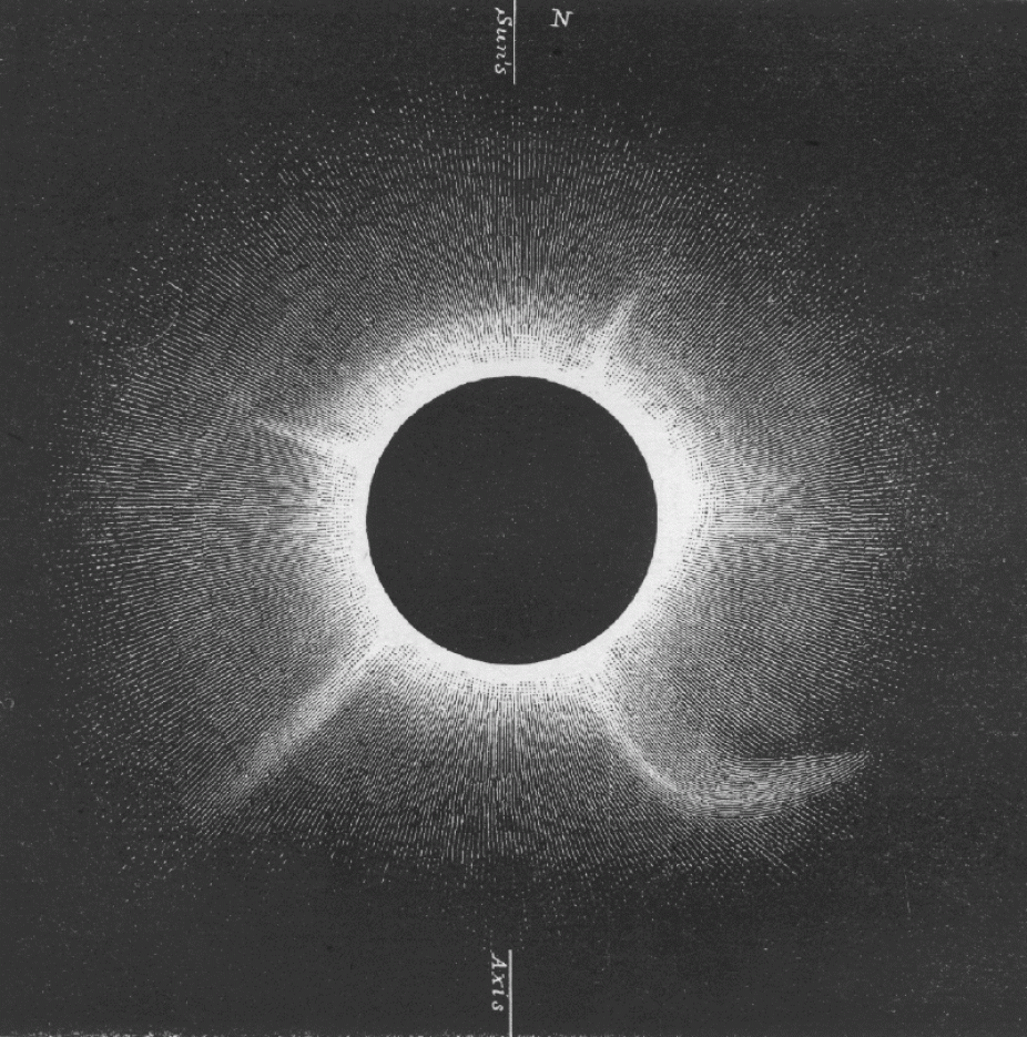
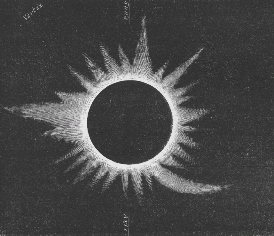
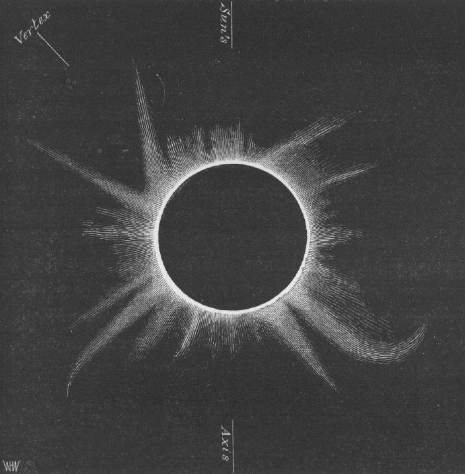
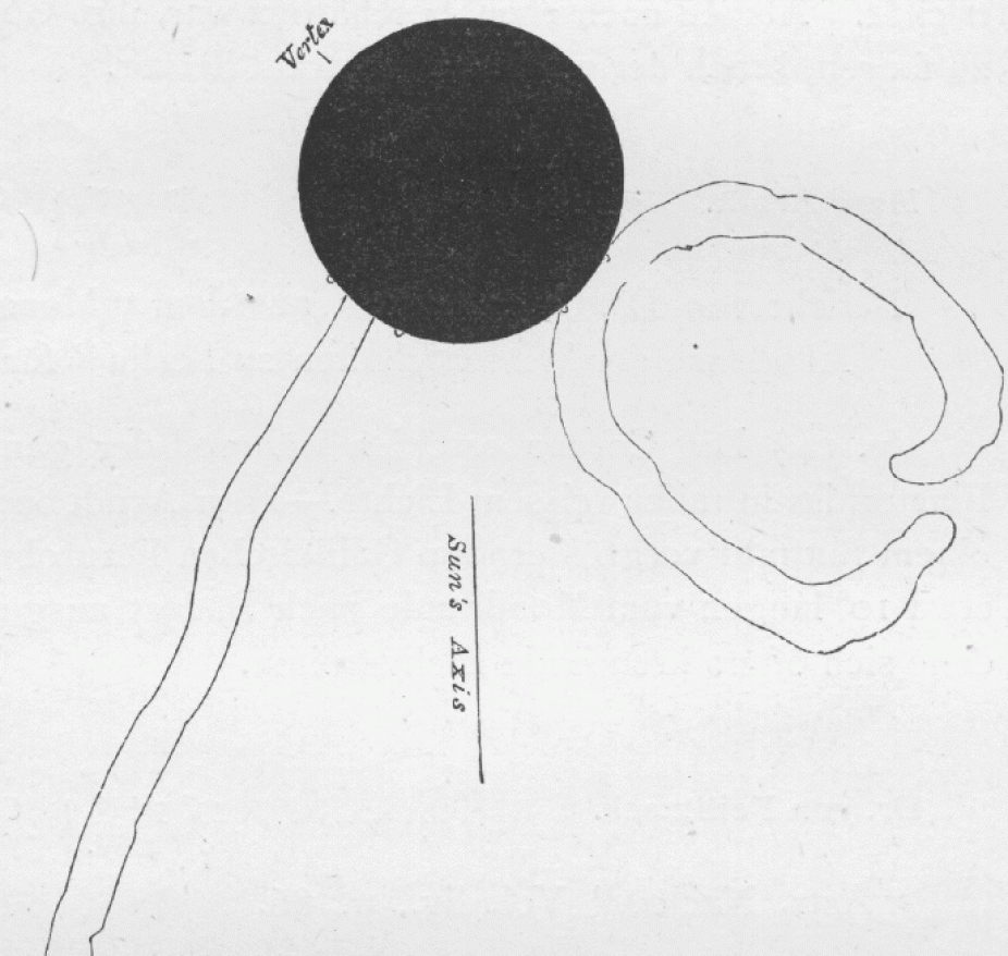
1860: First observations of a coronal mass ejection
The total solar eclipse of 18 July 1860 was probably the most thoroughly observed eclipse up to that time. These drawings include depictions of a peculiar feature in the SW (lower right) portion of the corona. Based on comparison with modern coronal observations, it is quite likely that these represent the first record of a Coronal Mass Ejection in progress.
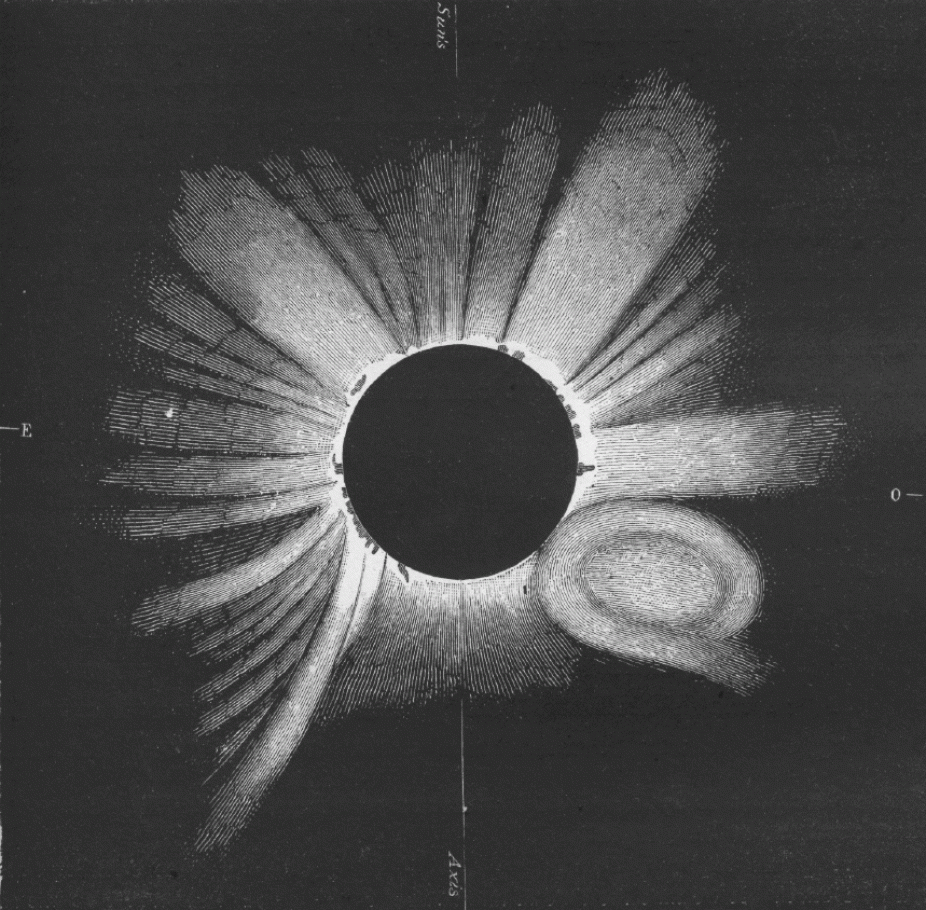
Drawing by G. Tempel
Drawing by von Feilitzsch
Drawing by F.A. Oom
Drawing by E.W. Murray
Drawing by F. Galton
Drawing by C. von Wallenberg
Drawings of the 1860 eclipse
(Reproduced from Ranyard, C.A, 1879, Mem. Roy. Astron. Soc., 41, 520, chap. 44.)
Today coronal mass ejections are known to represent one of the more energetic and geo-effective manifestations of solar activity, with up to 10 billion tons of material being ejected into interplanetary space at speeds reaching up to 1000 kilometer per second. For more detail on CMEs see slide 13 and slide 14 of the HAO slide set.
References and further readings
- Eddy, J.A. 1974, A Nineteenth-century Coronal Transient, in Astronomy and Astrophysics, 34, 235–240.
1881: The solar constant, again
Samuel Langley's base camp on California's Mt Whitney, July 1881. Some of Langley's instruments failed to arrive or arrived damaged, with the crucial spectral bolometer back in working order only by the end of August. The expedition was cut short on 8 September due to worsening observing conditions caused by the breakout of a series of wildfires elsewhere in California a few days earlier. Nonetheless, valuable data were collected.
Reproduced from: Eddy, J.A. 1990, J. Hist. Astron., 21, p. 115
By the second half of the nineteenth century, after various solar observing expedition to mountaintops, it was becoming increasingly clear that the Earth's atmosphere absorbs a significant portion of the sun's luminosity. Consequently, attempts at determining the solar constant were moved to the highest practical altitudes.
The American scientist Samuel Langley carried out the most elaborate attempt at determining the solar constant at the time, during an expedition to Mt Whitney, California, in July 1881. Using his recently invented bolometer (an instrument based on the varying electrical resistivity of metals with temperature), as well as other instruments, Langley carried out measurements at different wavelengths and at different altitudes, demonstrating the strong variation with wavelength of the absorption by Earth's atmosphere. However, the solar constant value he calculated at the time, 2903 Watt per square meters, is nearly a factor of two larger than the modern value (1367 W/m2), something apparently due to errors in the data reduction procedure, since Langley's later assistant Charles Abbot (1872–1973) obtained 1465 W/m2 with the original Mt Whitney data.
References and further readings
- Hufbauer, K. 1991, Exploring the Sun, The Johns Hopkins University Press.
- Eddy, J.A. 1990, Journal for the History of Astronomy, 21, p. 115.
- Foukal, P.V. 1990, Solar Astrophysics, John Wiley and Sons.
1908: The magnetic nature of sunspots
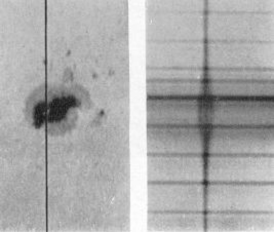
The magnetically-induced Zeeman splitting in the spectrum of a sunspot.
Reproduced from the 1919 paper by G.E. Hale, F. Ellerman, S.B. Nicholson, and A.H. Joy (in The Astrophysical Journal, vol. 49, pps. 153-178)
The study of sunspots and their 11-year cycle was finally put on a firm physical footing by the epoch-making work of George Ellery Hale (1868-1938) and collaborators in the opening decades of the twentieth century. In 1907–1908, by measuring the Zeeman splitting in magnetically sensitive lines in the spectra of sunspots, and detecting the polarization of the split spectral components, Hale provided the first unambiguous and quantitative demonstration that sunspots are the seats of strong magnetic fields (see also slide 4 and slide 5 of the HAO slide set). Not only was this the first detection of a magnetic field outside the Earth, but the inferred magnetic field strength, 3000 Gauss, is over a thousand times greater than the Earth's own magnetic field. It was subsequently realized that the pressure provided by such strong magnetic field would also lead naturally to the lower temperatures observed within the sunspots, as compared to the photosphere.
References and further readings
- Hale, G.E. 1908, On the probable existence of a magnetic field in sunspots, The Astrophysical Journal, 28, pps. 315–343
- Stix, M. 1989, The Sun, Springer.
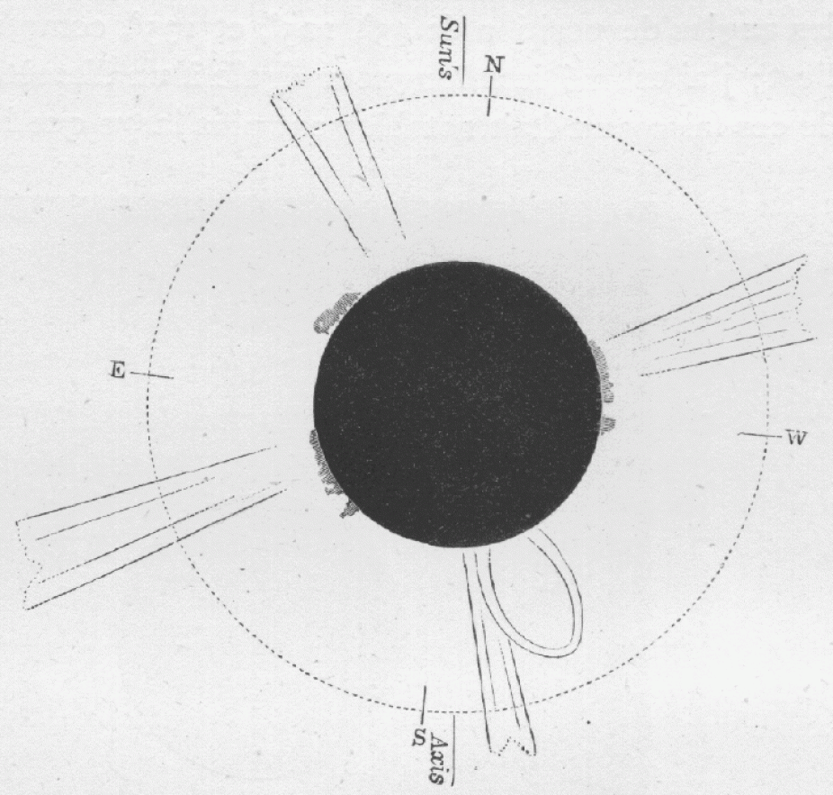
1919: The Sun's magnetic cycle
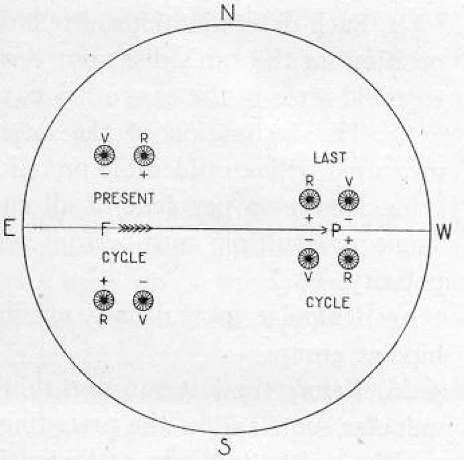
A diagram taken from the 1919 paper by G.E. Hale, F. Ellerman, S.B. Nicholson, and A.H. Joy, illustrating what is now known as Hale's polarity laws. This presented solid evidence for the existence of a well-organized large-scale magnetic field in the solar interior, which cyclically changes polarity approximately every 11 years.
The Astrophysical Journal, vol. 49, pps. 153–178
In the decade following his groundbreaking discovery of sunspot magnetic fields, George Ellery Hale and his collaborators went on to show that large sunspots pairs almost always (1) show the same magnetic polarity pattern in each solar hemisphere, (2) show opposite polarity patterns between the North and South solar hemispheres, and (3) these polarity patterns are reversed from one sunspot cycle to the next, indicating that the physical magnetic cycle has a period twice that of the sunspot cycle period. These empirical observations have stood the test of time and are known as "Hale's polarity Laws". Their physical origin is now known to be the operation of a large scale "hydromagnetic dynamo" within the solar interior, although the details of the process are far from adequately understood. Because the Sun's dynamo-generated magnetic field is ultimately responsible for all manifestations of solar activity (flares, coronal mass ejections, etc.), solar dynamo modeling remains a very active area of research in solar physics.
References and further readings
- Hale, G.E., Ellerman, F., Nicholson, S.B., and Joy, A.H. 1919, The Astrophysical Journal, 49, pps. 153–178
- Stix, M. 1989, The Sun, Springer.
1931: The Coronagraph
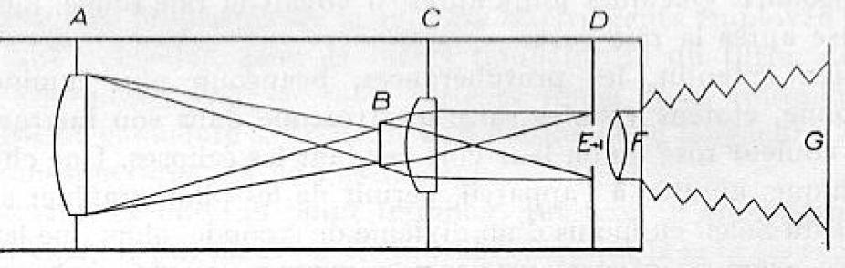
Bernard Lyot's coronagraph design. The occulting disk is at B, and the diaphragm and screen at D, E are needed to block stray light arising from diffraction at the primary lens and diaphragm A.
Reproduced from L'Astronomie, 66 (1952) (Fig. 113, p. 269)
Much of the remarkable progress made in understanding the Sun's outer atmosphere had been made through the use of observations carried out during total solar eclipses. The relative rarity of such eclipses, the cost and logistical difficulties of traveling to often remote location to observe them, the short duration of totality, as well as the frustrating vagaries of weather, motivated the search for a way to observe the corona at will and in full daylight. This was finally achieved in 1931 by the French solar physicist Bernard Lyot (1897–1952), who first designed an instrument now known as the coronagraph.
A coronagraph is nothing more than a telescope equipped with an occulting disk sized in such a way as to block out the solar disk. Although this may sound trivial, it turns out to be extremely difficult to achieve the needed accurate optical alignment and mechanical stability, without which stray light makes the viewing of the faint corona all but impossible. Lyot also managed to secure the first full daylight photographs of the corona. His success motivated others to replicate and modify his design, the most successful of these followers being Max Waldmeier at the ETH/Zürich, and Donald H. Menzel (1901–1976) at Harvard College Observatory. Here at HAO, we've designed and observed with many coronagraphs, such as Mk3/Mk4, K-Cor, and the coronagraph aboard the SMM satellite.
References and further readings
- D'Azambuja, L. 1952, L'oeuvre de Bernard Lyot, L'Astronomie, 66, 265–277.
- Hufbauer, K. 1991, Exploring the Sun, The Johns Hopkins University Press.